
Moltbot Guide 2026: Setup, Security & Safe Hosting Explained
Complete Moltbot tutorial: Learn what this viral AI assistant does, critical security risks, safe setup steps & why VPS hosting is essential for privacy.
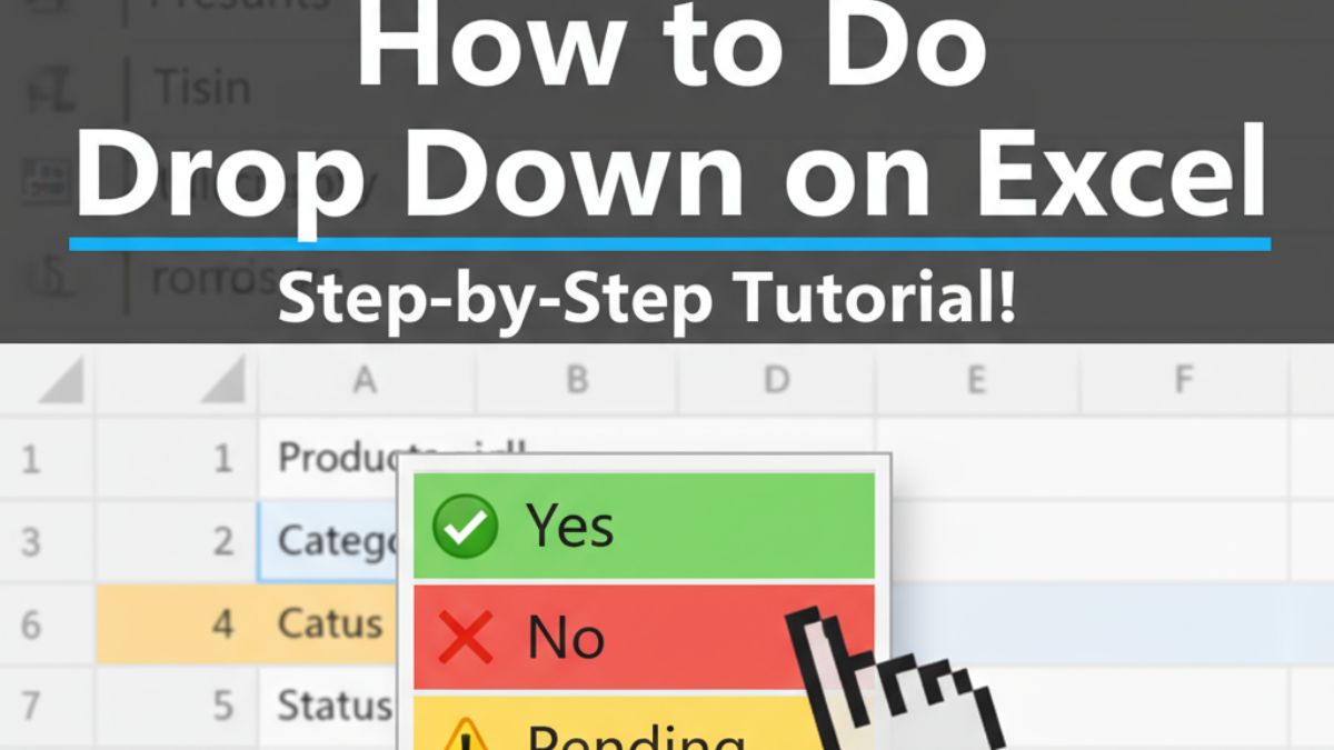
To create a drop-down list in Excel, select the cells, open Data > Data Validation, choose List under Allow, and type the options separated by commas or point Source at a range. This guide covers that method plus table-based dynamic lists, dependent drop-downs with INDIRECT, editing and removing lists, and fixes for the common errors.
Creating drop-down lists in Excel transforms cluttered spreadsheets into organized, error-free data systems. Whether you’re managing a sales pipeline, tracking project status, or building an expense tracker, Excel drop-down lists ensure data consistency and save hours of manual cleanup.
Drop-down lists help ensure consistency in data entry, which is particularly useful for forms and reports. Using drop-down lists and Data Validation saves time, improves data accuracy, and speeds up entry by streamlining the process and reducing manual errors.
This comprehensive guide walks you through every method to create drop down lists in Excel - from basic data validation to advanced dependent lists with VBA. You’ll learn techniques that work across Excel 365, Excel 2021, Excel 2019, and Excel for Mac, with real-world examples from small business owners, project managers, and financial analysts.
By the end, you’ll master:
Basic drop-down creation using data validation
Dynamic lists that update automatically with Excel tables
Dependent drop-downs (like State → City selections)
Multiple selection drop-downs with VBA code
Color-coded visual indicators
Mobile compatibility tips for Excel app
Let’s dive in with the fundamentals, then progress to advanced automation techniques.
An Excel drop-down list (also called a data validation list) appears as a clickable arrow icon in a cell. When clicked, it reveals predefined choices, restricting user input to approved options from a predefined list instead of allowing free-form typing.
This feature leverages Excel’s Data Validation tool, found under the Data tab, to create interactive spreadsheets that:
Prevent data entry errors (no more “Complted” instead of “Completed”)
Speed up data input by 40-60% (users click instead of type)
Maintain consistency across teams and departments
Enable advanced formulas that rely on standardized inputs
In a project management tracker, a drop-down might offer three status options:
In Progress
Completed
On Hold
This ensures every team member uses identical terminology, making filtered reports and pivot tables accurate.
Character limit: 255 characters per item
Item limit: Practically unlimited via cell references (tested up to 10,000 items)
Platform support: Windows, Mac, Excel Online, iOS/Android apps
Compatibility: Excel 2010 and newer (including Office 365/Microsoft 365)
Pro tip: Keep visible lists under 20 items for usability, longer lists benefit from searchable drop-downs using combo boxes (covered in Method 5).
To create a drop-down list in Excel, you need to use the Data Validation feature.
This fundamental approach works in all Excel versions and takes less than 2 minutes.
Step 1: Select the cell or range where you want the drop-down.
Step 2: Go to the Data tab and select Data Validation.
Step 3: The Data Validation dialog box will appear. In the Allow box, choose List. In the Source box, enter the options you want to appear in your drop-down. You can create a drop-down list by typing the items directly into the Source box, separated by commas.
Step 1: Select Your Target Cell(s)
Open your Excel workbook and click the cell where the drop-down should appear. For multiple rows, highlight the entire range, for example, B2:B100 for a 100-row project tracker.
Keyboard shortcut: Click B2, then press Ctrl + Shift + Down Arrow to select to the last row with data.
Step 2: Open Data Validation
Navigate to the Data tab on the Excel ribbon (top menu bar). In the Data Tools group, click Data Validation.
Alternative access: Press Alt + D + L (Windows) to open Data Validation directly.
Step 3: Configure List Settings
A dialog box titled "Data Validation" opens with three tabs: Settings, Input Message, and Error Alert.
In the Settings tab:
Under Allow, select List from the dropdown menu
In the Source box, enter your options separated by commas:
High,Medium,LowImportant: No spaces after commas unless you want spaces in your options
Check Ignore blank if you want to allow empty cells (recommended for optional fields)
Keep In-cell dropdown checked (this shows the arrow icon)
Step 4: Add Input Message (Optional but Recommended)
Switch to the Input Message tab:
Title: "Select Priority Level"
Input message: "Choose High, Medium, or Low from the dropdown list"
This creates a helpful tooltip that appears when users click the cell, reduces confusion by 75% in shared workbooks.
Step 5: Configure Error Alert
On the Error Alert tab:
Style: Stop (shows a red X icon)
Title: "Invalid Entry"
Error message: "Please select an option from the dropdown list. Custom entries are not allowed."
Style options explained:
Stop (recommended): Prevents invalid entries completely
Warning: Shows a warning but allows override
Information: Shows a message but doesn't restrict entry
Step 6: Apply and Test
Click OK. A small drop-down arrow appears in your selected cell(s).
Testing:
Click the arrow, your options (High, Medium, Low) should display
Try typing invalid text, the error alert should block it
Select each option to verify they appear correctly
To extend the drop-down to additional cells without re-creating it:
Select the cell with the drop-down (e.g., B2)
Copy it: Ctrl + C (Windows) or Cmd + C (Mac)
Select target cells (e.g., B3:B100)
Right-click → Paste Special → Validation
You can also apply data validation to all the cells in a range to ensure consistent data entry across the worksheet. This is especially useful when you want every cell in a column or table to use the same drop-down options.
This copies only the validation rules, preserving existing data in those cells.
Common mistake: Using regular paste (Ctrl + V) overwrites cell contents. Always use Paste Special > Validation for drop-downs.
Best for: Short lists of 3-10 items where you want to quickly create a drop down menu
This method embeds options directly in the Data Validation dialog, perfect for status indicators, priority levels, or yes/no fields. It's an ideal way to add a drop down menu in Excel for short lists, allowing you to enter options directly without referencing a separate data range.
Following the basic steps above, in the Source box, type comma-separated values:
New,In Progress,Under Review,Approved,RejectedFastest setup (no additional cells needed)
Self-contained (works when cells are deleted)
Easy to understand for Excel beginners
Tedious to edit (must reopen Data Validation each time)
Not scalable for lists exceeding 10 items
No dynamic updates (must manually update each drop-down)
Case sensitivity: Excel treats "High" and "high" as different entries, but drop-downs aren't case-sensitive by default. Add this formula to adjacent cells if exact case matters:
excel
=EXACT(B2,"High")Special characters: Avoid commas in item names (use semicolons as separators if your regional settings support it: File > Options > Advanced > Editing options > Use system separators).
Excel for Mac: Process identical to Windows, use Command instead of Ctrl for shortcuts.
Best for: Lists that change occasionally (10-50 items)
This approach stores list items in worksheet cells, allowing easy updates without reopening Data Validation. By referencing a cell range, you can use a predefined list for your drop-down, which helps standardize data entry, reduce errors, and improve usability in your spreadsheet.
Advanced Techniques:
For even more flexibility, define a named range for your list items (Formulas > Name Manager). Using named ranges can make referencing your drop-down list items easier and more user-friendly. This also allows you to move or expand your list without breaking the drop-down.
Step 1: Create Your Source List
In a separate area of your worksheet (or hidden sheet), enter items in a vertical column:
|
A |
B |
|---|---|
|
1 |
Apple |
|
2 |
Banana |
|
3 |
Orange |
|
4 |
Grape |
|
5 |
Mango |
Pro tip: Use a hidden sheet for cleaner workbooks:
Right-click sheet tab → Hide
Reference as =Sheet2!$A$1:$A$5
Step 2: Set Up Data Validation
Select target cells (e.g., C2:C50)
Open Data Validation (Alt + D + L)
In Source, enter: =$A$1:$A$5
Important: Use absolute references ($A$1:$A$5) so the range doesn't shift when copying to other cells.
Step 3: Test Dynamic Updates
Change "Apple" to "Pineapple" in cell A1, the drop-down updates immediately (no need to reapply validation).
Dynamic Range Expansion:
If your list grows, use this formula to auto-adjust the range:
excel
=$A$1:INDEX($A:$A,COUNTA($A:$A))This counts filled cells and extends the range automatically.
Named Ranges:
For easier reference:
Select A1:A5
Press Ctrl + Shift + F3
Name it "FruitList"
In Source: =FruitList
Excel Online (Browser Version): Ranges work identically, but collaborative edits may have a 1-2 second delay before drop-downs update for other users.
Best for: Growing lists (50+ items) that need automatic expansion
Using an excel table allows you to create a dynamic drop down list in Excel that automatically updates as you add or remove items. Excel Tables (structured references) auto-expand when you add rows, eliminating manual range updates.
Select your source list and press Ctrl+T to convert it to an Excel Table.
You can store your items in an Excel table to create a dynamic drop-down list that automatically updates when new items are added.
Auto-expansion: Add items to the table bottom, drop-downs update instantly
Structured references: Formulas use table names, not cell addresses
Filtering built-in: Users can filter drop-down sources easily
Professional appearance: Formatted with alternating row colors
Step 1: Convert Your List to a Table
Select your list items (e.g., A1:A10 including header "Fruits")
Press Ctrl + T (or Insert > Table)
Check "My table has headers" → OK
Excel adds formatting and filter arrows
Step 2: Name Your Table
Click anywhere in the table
Table Design tab appears on ribbon
In Table Name box (left side), enter: FruitList
Naming rules:
No spaces (use underscores: Fruit_List)
Must start with letter or underscore
Maximum 255 characters
Step 3: Create Drop-Down with Structured Reference
Select drop-down destination cells (e.g., D2:D50)
Open Data Validation
In Source, enter:
excel
=FruitList[Fruits](Replace "Fruits" with your column header)
Step 4: Test Auto-Expansion
Click the last row in your table
Press Tab to add a new row
Enter "Strawberry"
Check your drop-down"Strawberry" appears automatically
Excel 365/2021: Full support with dynamic arrays
Excel 2019/2016: Supported (no dynamic arrays, but tables work)
Excel 2013 and older: Convert table to range first if issues occur
Keyboard shortcut: Ctrl + Shift + L toggles table filters (useful for sorting drop-down source data).
Best for: Related choices like Country → State → City, or Category → Subcategory
To set up dependent (cascading) drop-downs in Excel, you must first create the first drop down list, which serves as the main category. This involves selecting the cells, using data validation, and referencing a source range such as '=Category'. After establishing the main category list, you then set up subcategory lists for each main category. Dependent drop-downs change options based on previous selections, critical for complex forms and databases.
Primary dropdown: Product Category (Electronics, Clothing, Home Goods)
Dependent dropdown: Specific Products (changes based on category selected)
Step 1: Organize Your Data
Create this structure on a worksheet:
|
A |
B |
C |
|---|---|---|
|
Categories |
Electronics |
Clothing |
|
Electronics |
Laptop |
T-Shirt |
|
Clothing |
Smartphone |
Jeans |
|
Home Goods |
Tablet |
Jacket |
|
Headphones |
Sneakers |
Step 2: Create Named Ranges
For each category:
Select B2:B5 (Electronics items)
Formulas tab → Define Name
Name: Electronics → OK
Repeat for "Clothing" (C2:C5) and "Home_Goods" (use underscore for spaces).
Step 3: Primary Drop-Down
Select cell E2 (category selection)
Data Validation → Source: =Categories!$A$2:$A$4
Step 4: Dependent Drop-Down with INDIRECT
Select cell F2 (product selection)
Data Validation → Source:
excel
=INDIRECT(E2)How it works: When E2 = "Electronics", INDIRECT converts the text "Electronics" into the named range reference, pulling items from B2:B5.
If categories have spaces ("Home Goods"), use SUBSTITUTE:
excel
=INDIRECT(SUBSTITUTE(E2," ","_"))This converts "Home Goods" to "Home_Goods" for the named range.
For Excel 365 only, use FILTER for more flexibility:
excel
=FILTER(Products[Product], Products[Category]=E2)This doesn't require named ranges, just a table with columns "Category" and "Product".
#REF! Error:
Named range doesn't exist or is misspelled
Use Formulas > Name Manager to verify names
Drop-down shows #NAME?:
INDIRECT can't find the named range
Check for spaces or special characters in cell E2
Items don't appear:
Named range is empty
Ensure primary selection matches named range exactly (case-insensitive but spelling must match)
Multi-level dependents (3+ levels): Use nested INDIRECT or create a master table with all relationships, see advanced tutorial [link to future guide].
Best for: Skills tracking, tag systems, or any field needing multiple choices
Standard Excel drop-downs allow only one selection. For multi-select (e.g., selecting "Excel, PowerPoint, Word" for skill tracking), you need VBA (Visual Basic for Applications).
File format: Save as .xlsm (Excel Macro-Enabled Workbook)
Security: Enable macros when opening (some companies block this)
Compatibility: VBA doesn't work in Excel Online (browser version)
Step 1: Enable Developer Tab
File > Options
Customize Ribbon
Check Developer in the right column
Click OK
Step 2: Create Basic Drop-Down First
Set up a normal drop-down in cell B2 with options:
Excel, Word, PowerPoint, Outlook, TeamsStep 3: Open VBA Editor
Press Alt + F11 (Windows) or Option + F11 (Mac)
Step 4: Insert Module
In VBA editor: Insert > Module
Paste this code:
vba
Private Sub Worksheet_Change(ByVal Target As Range)
    ' Multi-select drop-down for column B
    Dim Oldvalue As String
    Dim Newvalue As String

    ' Only run for column B, rows 2-100
    If Target.Column = 2 And Target.Row >= 2 And Target.Row <= 100 Then
        Application.EnableEvents = False

        Newvalue = Target.Value
        Application.Undo
        Oldvalue = Target.Value

        Target.Value = Newvalue

        If Oldvalue = "" Then
            ' First selection
            Target.Value = Newvalue
        Else
            ' Check if item already selected
            If InStr(1, Oldvalue, Newvalue) = 0 Then
                ' Add new item with comma separator
                Target.Value = Oldvalue & ", " & Newvalue
            Else
                ' Item already exists, don't add
                Target.Value = Oldvalue
            End If
        End If

        Application.EnableEvents = True
    End If
End Sub
Step 5: Place Code in Correct Location
In the VBA editor's Project Explorer (left panel)
Double-click the worksheet name (e.g., "Sheet1")
Paste the code in the window that opens
Important: Don't paste in a Module, paste in the Worksheet object
Step 6: Save and Test
Press Alt + Q to close VBA editor
Save as .xlsm format
Click cell B2's drop-down
Select "Excel" → appears in cell
Click drop-down again, select "Word" → cell now shows "Excel, Word"
This code doesn't include removal functionality. To remove an item:
Manually delete the unwanted item from the cell text
Or clear the entire cell and re-select
Advanced version with removal: Available in downloadable template [link at end].
For Excel Online or macro-restricted environments:
Developer tab → Insert → Check Box (Form Controls)
Place checkboxes next to item labels
Link each checkbox to a cell: Right-click checkbox → Format Control → Cell link: C2
Use formula to concatenate checked items:
excel
=TEXTJOIN(", ", TRUE, IF(C2:C6=TRUE, A2:A6, ""))(Array formula: Enter with Ctrl + Shift + Enter in Excel 2019 and older)
Pros: Works everywhere, no security concerns
Cons: Takes more space, less elegant than drop-downs
Best for: Status tracking, priority indicators, or any categorization needing visual cues
Adding colors to drop-down selections improves scannability by 60%, users spot "red = urgent" instantly.
Step 1: Create Standard Drop-Down
Set up a drop-down in column B with options:
High, Medium, LowStep 2: Apply Conditional Formatting
Select cells with drop-downs (e.g., B2:B50)
Home tab → Conditional Formatting → New Rule
Select Use a formula to determine which cells to format
Step 3: Create Rules for Each Option
For "High" priority (Red background):
Formula: =$B2="High"
Format: Click Format → Fill tab → Red color
Click OK → OK
For "Medium" priority (Yellow background):
New Rule again
Formula: =$B2="Medium"
Format: Yellow fill
For "Low" priority (Green background):
Formula: =$B2="Low"
Format: Green fill
Important: Use =$B2 (column absolute, row relative) so formatting applies to entire column when you select B2:B50.
For data that implies progression:
Select cells
Conditional Formatting → Icon Sets → 3 Arrows
Manage Rules → Edit the rule
Set thresholds:
Green arrow: "Completed"
Yellow arrow: "In Progress"
Red arrow: "Not Started"
For color-blind users (8% of males, 0.5% of females):
Combine colors with patterns: Format Cells → Fill tab → Pattern Style
Add text indicators: Use formulas like:
excel
=B2&" - "&IF(B2="High","🔴","")Add cell comments: Review → New Comment with text descriptions
Screen reader compatibility: Comments (not notes) are read aloud by accessibility software.
Quick method:
Select cell with drop-down
Alt + D + L (opens Data Validation)
Modify Source, messages, or alerts
Click OK
Bulk editing:
Select all cells with the drop-down (use Ctrl + Click for non-contiguous cells)
Open Data Validation, changes apply to all selected cells
Modify as needed
Single cell:
Select cell
Data Validation → Clear All
Multiple cells:
Select range
Data Validation → Clear All
Cells retain their current values, only the drop-down arrow disappears
Method 1: Paste Special (Recommended)
Select source cell with drop-down
Ctrl + C
Select target cell(s)
Right-click → Paste Special → Validation
Method 2: Format Painter
Select source cell
Home tab → Format Painter (paintbrush icon)
Click target cell(s)
Note: Also copies other formatting (colors, fonts)
Problem: Sorting breaks cell references in Source field
Solution: Use Excel Tables (Method 3) or Named Ranges (Method 2), both maintain references after sorting.
Lock source range:
Select source cells → Right-click → Format Cells
Protection tab → Check Locked
Review tab → Protect Sheet
Allow users to "Select locked cells" and "Sort"
Causes and fixes:
✓ "In-cell dropdown" unchecked
Solution: Data Validation → Check In-cell dropdown
✓ Merged cells
Solution: Select cells → Home → Merge & Center → Unmerge Cells
Create drop-down after unmerging
✓ Cell protection
Solution: Review → Unprotect Sheet (if password-protected)
Causes:
✓ Blank cells in source range
Solution: Use =A1:A10 instead of =A:A (entire column)
Or clean data: =TRIM(CLEAN(A1:A10))
✓ Hidden rows in source
Solution: Unhide all rows in source range
Or use formula: =FILTER(A1:A10, A1:A10<>"") (Excel 365)
Causes:
✓ Named range misspelled or deleted
Solution: Formulas → Name Manager → Verify names match
Check for spaces (use underscore in names: New_York)
✓ INDIRECT references deleted range
Solution: Recreate named range exactly as referenced
Causes:
✓ Code in wrong location
Solution: Must be in Worksheet object, not Module
Copy code, delete module, paste in Sheet1 (VBA Project Explorer)
✓ Macros disabled
Solution: File → Options → Trust Center → Trust Center Settings → Macro Settings → Enable macros
✓ Wrong file format
Solution: Save as .xlsm, not .xlsx
Symptoms: Drop-down takes 3+ seconds to open
Solutions:
✓ Limit list to 100 items
For 100+ items, use searchable combo box (ActiveX control)
✓ Reduce dependent drop-down complexity
Avoid 3+ levels of dependents
Use database queries instead (Power Query)
✓ Disable auto-calculate
Formulas → Calculation Options → Manual
Press F9 to recalculate when needed
Excel for Mac differences:
✓ Keyboard shortcuts
Windows Alt + D + L → Mac Cmd + Option + V (not direct equivalent, use menu)
✓ Some VBA needs modifications
Replace Application.EnableEvents with error handlers
Test macros thoroughly on Mac before deploying
✓ ActiveX controls unavailable
Use Form Controls instead (checkboxes, combo boxes)
What works:View and select from existing drop-downs
Basic data validation editing
Cell range references
What doesn't work:VBA macros (multi-select code)
Creating dependent drop-downs (formula-based)
Advanced conditional formatting
iOS (iPhone/iPad):
Tap cell
Data button (bottom toolbar)
Data Validation
Enter items in Source box (comma-separated)
Tap Done
Android:
Tap cell
Edit → Data
Data Validation
Enter source
Tap checkmark
Limitation: Can't reference cell ranges on mobile, must type items directly.
Workaround: Create drop-downs on desktop, sync via OneDrive/SharePoint, then use mobile app only for data entry (not creation).
Better alternative: Use web.office.com on mobile browser
Full desktop functionality
Supports cell references and tables
No VBA, but dependent drop-downs work (INDIRECT)
Responsive design: Works on tablets (iPad, Android) with larger screens, phone browsers can be challenging for complex editing.
Scenario: A New York City freelance consultant needs to track monthly business expenses with category and vendor analysis.
|
Date |
Category |
Subcategory |
Vendor |
Amount |
Notes |
|---|---|---|---|---|---|
|
1/15/2026 |
Office |
Software |
Adobe |
$52.99 |
Creative Cloud |
|
1/16/2026 |
Marketing |
Advertising |
|
$250.00 |
Ads Campaign |
Column B (Category) - Primary Drop-Down:
Office, Marketing, Travel, Equipment, Professional ServicesColumn C (Subcategory) - Dependent Drop-Down:
Office → Software, Supplies, Furniture
Marketing → Advertising, Events, Content Creation
Travel → Airfare, Hotel, Ground Transportation
Equipment → Computer, Phone, Accessories
Professional Services → Legal, Accounting, Consulting
Column D (Vendor) - Searchable Combo Box: For 50+ vendors, use an ActiveX Combo Box (desktop only):
Developer → Insert → ActiveX Combo Box
Right-click → Properties
ListFillRange: =VendorList (named range)
LinkedCell: D2
Column E (Amount) - Data Validation with Number Constraints:
Decimal allowed, between $0.01 and $10,000Total by Category:
excel
=SUMIF($B:$B, "Marketing", $E:$E)Count Transactions by Subcategory:
excel
=COUNTIF($C:$C, "Software")Pivot Table Recommendations:
Rows: Category, Subcategory
Values: Sum of Amount
Filters: Date (by month)
Create a searchable drop-down that filters as you type:
Setup:
Name your list range: ProductList
In a helper column, use:
excel
=FILTER(ProductList, ISNUMBER(SEARCH(D2, ProductList)))(Where D2 is user's search term)
Create drop-down sourcing this formula result
Limitation: Requires Excel 365 with dynamic array support
Step 1: Insert ActiveX Combo Box
Developer → Insert → ActiveX Controls → Combo Box
Step 2: Properties
ListFillRange: Your source range (e.g., $A$1:$A$100)
LinkedCell: Target cell (e.g., $B$2)
MatchEntry: 2 - fmMatchEntryComplete
Step 3: Enable auto-complete
Right-click combo box → View Code
Paste:
vba
   Private Sub ComboBox1_Change()
       ComboBox1.DropDown
   End Sub
Result: As user types "App", combo shows "Apple", "Application", etc.
Use case: Databases with 500+ items (customer names, product SKUs)
Create a template: Save workbook with pre-built drop-downs as .xltx (Excel Template)
File → Save As → Excel Template
Store in shared OneDrive/SharePoint folder
Team members open template to start new files with consistent drop-downs
Lock validation while allowing data entry:
Select cells WITHOUT drop-downs → Format Cells → Protection → Uncheck Locked
Select cells WITH drop-downs → Keep Locked checked
Review → Protect Sheet
In Allow users to: Check Select unlocked cells and Format cells
Uncheck Select locked cells (prevents changing drop-downs)
Result: Users can enter data everywhere except drop-down cells, but CAN use the drop-downs.
Track who changed what (Excel 365 only):
Save file to OneDrive/SharePoint
Review → Track Changes (in co-authoring mode)
View history: File → Info → Version History
Alternative: Use Power Automate (formerly Flow) to log changes to SharePoint list.
Include instructions tab:
Sheet named "README"
Explain each drop-down's purpose
List dependencies (Category → Subcategory)
Contact info for questions
Embed help in workbook:
Developer → Insert → Button
Link to macro that opens MsgBox with instructions
Or hyperlink to company wiki/SharePoint page
|
Action |
Windows |
Mac |
|---|---|---|
|
Open Data Validation |
Alt + D + L |
No direct shortcut (use menu) |
|
Open drop-down |
Alt + Down Arrow |
Option + Down Arrow |
|
Select from drop-down |
Type first letter, then Enter |
Same |
|
Clear validation |
Alt + D + L, then Delete, Enter |
Use menu |
|
Copy validation |
Ctrl + C, then Alt + E + S + N |
Cmd + C, then menu |
|
Paste Special Validation |
After copying: Alt + E + S + N |
After copying: Cmd + Ctrl + V (limited) |
Time-saving tip: Memorize Alt + Down Arrow to open drop-downs without mouse, saves 2-3 seconds per entry (adds up over 100+ entries).
Excel's Data Validation isn't just for lists, explore these options:
Use case: Quantity fields, age entry
Setup:
Allow: Whole number
Data: between
Minimum: 1, Maximum: 100
Error message: "Enter quantity between 1 and 100"
Use case: Booking systems, project deadlines
Setup:
Allow: Date
Data: greater than
Start date: =TODAY()
Result: Only future dates accepted
Use case: Product codes, zip codes
Setup:
Allow: Text length
Data: equal to
Length: 5 (for 5-digit zip codes)
Use case: Email address format
Setup:
Allow: Custom
Formula:
excel
=AND(ISNUMBER(FIND("@",B2)), ISNUMBER(FIND(".",B2)))Result: Blocks entries without @ and . (basic email check)
Drop-down lists transform Excel from a static grid into an interactive data system. Whether you're building a simple priority tracker or a complex multi-level inventory database, these methods cover every scenario:
Quick reference:
Method 1 (Direct Entry): Fast, 3-10 items, rarely changes
Method 2 (Cell Range): Editable, 10-50 items, occasional updates
Method 3 (Tables): Dynamic, 50+ items, grows automatically
Method 4 (Dependent): Related choices (Category → Item)
Method 5 (VBA Multi-Select): Multiple selections per cell
Method 6 (Color-Coded): Visual priority indicators
Use VBA code (Method 5 above) to enable multi-select functionality. Standard Excel drop-downs only allow one choice. The VBA script appends selections with comma separators (e.g., "Excel, Word, PowerPoint"). Steps: Enable Developer tab Press Alt + F11 for VBA editor Paste multi-select code in Worksheet object (not Module) Save as .xlsm file No-VBA alternative: Use checkboxes with TEXTJOIN formula for concatenation.
Apply the dependent drop-down validation to an entire column range (e.g., F2:F100). The INDIRECT formula adjusts automatically for each row: excel =INDIRECT($E2) Use column absolute ($E) but row relative (2) so the formula references E2, E3, E4, etc., as you copy down. Excel 365 alternative: excel =FILTER(Products[Product], Products[Category]=$E2)
Use SUMIF to sum based on drop-down selections: excel =SUMIF($B:$B, "High", $C:$C) Explanation: $B:$B - Column with drop-downs (criteria range) "High" - Value to match (or reference a cell like E2) $C:$C - Column with numbers to sum Advanced: Sum multiple criteria: excel =SUMIFS($C:$C, $B:$B, "High", $D:$D, "Completed")
Select cells with drop-down Data Validation (Alt + D + L) Modify Source field Click OK Existing cell values remain unchanged, only the available options update. Bulk edit: Select all cells with the drop-down before opening Data Validation (use Ctrl + Click for non-adjacent cells).
Yes, process is similar: Google Sheets steps: Select cell(s) Data → Data validation Criteria: List of items Enter comma-separated values or range Check Show dropdown list in cell Save Key difference: Google Sheets uses "List from a range" (similar to Excel's cell reference method) but doesn't support VBA. For dependent drop-downs, use INDIRECT the same way.
Reference the other sheet in your Source field: excel =Sheet2!$A$1:$A$10 If sheet name has spaces: excel ='Product List'!$A$1:$A$10 Pro tip: Use named ranges to avoid complex references: Go to Sheet2, select A1:A10 Formulas → Define Name → "Products" Back on Sheet1, Source: =Products
The cells still contain the old values, drop-down only controls NEW entries. To clear: Option 1: Select cells → Delete key (clears contents) Option 2: Find and replace: Ctrl + H Find what: Old value Replace with: (leave blank) Replace All Note: This doesn't affect the drop-down options themselves, those update when you edit the Source range.
Not natively in Excel. Workarounds: Method 1: Conditional Formatting with Icons Use icon sets based on drop-down value (Method 6 above) Limited to Excel's built-in icons Method 2: VBA UserForm Create custom form with image buttons Advanced, requires VBA programming Method 3: Power Apps Build custom app integrated with Excel Overkill for most use cases Recommendation: Use text drop-downs with descriptive labels or icons via conditional formatting.
 Tutorials and How-To Guides
Complete Moltbot tutorial: Learn what this viral AI assistant does, critical security risks, safe setup steps & why VPS hosting is essential for privacy.
 Tutorials and How-To Guides
Learn how to connect Google Cloud Storage to n8n workflows. Complete setup guide with OAuth2 configuration, bucket creation, and automation examples.
 Tutorials and How-To Guides
Learn how to set up Redis as your n8n storage database. Step-by-step configuration guide with screenshots, troubleshooting tips, and best practices for 2026.